Foldy–Wouthuysen transformation
The Foldy-Wouthuysen (FW) transformation (after Lesley L. Foldy and Siegfried A. Wouthuysen) is a unitary transformation on a fermion wave function of the form:
 (1)
(1)
where the unitary operator is the 4x4 matrix:
 . (2)
. (2)
Above,  is the unit vector oriented in the direction of the fermion momentum. The above are related to the Dirac matrices by
  and
and  , with i=1,2,3. A straightforward series expansion applying the commutativity properties of the Dirac matrices demonstrates that (2) above is true. The inverse
  , so it is clear that
  , where
  is a 4x4 identity matrix.
Foldy-Wouthuysen Transformation of the Dirac Hamiltonian for a Free Fermion
This transformation is of particular interest when applied to the free-fermion Dirac Hamiltonian operator  in bi-unitary fashion, in the form:
 (3)
(3)
Using the commutativity properties of the Dirac matrices, this can be massaged over into the double-angle expression:
 (4)
(4)
This factors out into:
 (5)
(5)
Choosing a Particular Representation: Newton-Wigner
Clearly, the FW transformation is a continuous transformation, that is, one may employ any value for  which one chooses. Now comes the distinct question of choosing a particular value for , which amounts to choosing a particular transformed representation.
One particularly important representation, is that in which the transformed Hamiltonian operator  is diagonalized. Clearly, a completely diagonalized representation can be obtained by choosing such that the
  term in (5) is made to vanish. Such a representation is specified by defining:
 (6)
(6)
so that (5) is reduced to the diagonalized (this presupposes that  is taken in the Dirac-Pauli representation (after Paul Dirac and Wolfgang Pauli) in which it is a diagonal matrix):
 (7)
(7)
By elementary trigonometry, (6) also implies that:
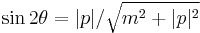 and
and 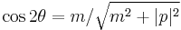 (8)
(8)
so that using (8) in (7) now leads following reduction to:
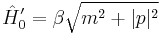 (9)
(9)
This calculation can be examined in further detail in the following link.
Prior to Foldy and Wouthuysen publishing their transformation, it was already known that (9) is the Hamiltonian in the Newton-Wigner (NW) representation (named after Theodore Duddell Newton and Eugene Wigner) of the Dirac equation. What (9) therefore tells us, is that by applying a FW transformation to the Dirac-Pauli representation of Dirac's equation, and then selecting the continuous transformation paramater so as to diagonalize the Hamiltonian, one arrives at the NW representation of Dirac's equation, because NW itself already contains the Hamiltonian specified in (9). See this link
If one considers an "on shell" mass -- fermion or otherwise -- given by  , and employs a Minkowski metric tensor for which
  , it should be apparent that the expression
 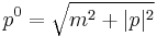 is equivalent to the
  component of the energy-momentum vector
  , so that (9) is alternatively specified rather simply by
  .
.
Correspondence Between the Dirac-Pauli and Newton-Wigner Representations, for an "At Rest" Fermion
Now let us consider a fermion "at rest," which we may define in this context as a fermion for which  . From (6) or (8), this means that
  , so that
  , and, from (2), that the unitary operator
  . Therefore, any operator
  in the Dirac-Pauli representation upon which we perform a bi-unitary transformation, will be given, for an "at rest" fermion, by:
 . (10)
Contrasting the original Dirac-Pauli Hamiltonian Operator with the NW Hamiltonian (9), we do indeed find the "at rest" correspondence:
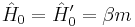 (11)
(11)
The Velocity Operator in the Dirac-Pauli Representation
Now, let us consider the velocity operator. To obtain this operator, we must commute the Hamiltonian operator  with the canonical position operators
  , i.e., we must calculate
 ![\hat{v_i}\equiv i[\hat{H}_0,x_i]](/2012-wikipedia_en_all_nopic_01_2012/I/bb8fb181a889b230d1f70726672a5271.png) . One good way to approach this calculation, is to start by writing the scalar rest mass
. One good way to approach this calculation, is to start by writing the scalar rest mass  as
as 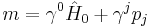 , and then to mandate that the scalar rest mass commute with the . Thus, we may write:
![0=[m,x_i]=[(\gamma^0\hat{H}_0%2B\gamma^jp_j),x_i]=[\gamma^0\hat{H}_0,x_i]%2Bi\gamma_i](/2012-wikipedia_en_all_nopic_01_2012/I/e63c389ee5166ff31f4d9d87802f5022.png) (12)
(12)
where we have made use of the Heisenberg canonical commutation relationship ![[x_i,p_j]=-i\eta_{ij}](/2012-wikipedia_en_all_nopic_01_2012/I/b4bb04a3d5a5c0353ff82c26fd0ad7b3.png) to reduce terms. Then, multiplying from the left by
to reduce terms. Then, multiplying from the left by  and rearranging terms, we arrive at:
![\frac{\hat{dx_i}}{dt}=\hat{v_i}\equiv i[\hat{H}_0,x_i]=\alpha_i](/2012-wikipedia_en_all_nopic_01_2012/I/ed5fd493b0d66abec608a6208ffa7393.png) (13)
(13)
Because the canonical relationship ![i[\hat{H}_0,\hat{v}_i] \ne 0](/2012-wikipedia_en_all_nopic_01_2012/I/766a36d74d8ce618e113494c454d4807.png) , the above provides the basis for computing an inherent, non-zero acceleration operator, which specifies the oscillatory motion known as Zitterbewegung.
, the above provides the basis for computing an inherent, non-zero acceleration operator, which specifies the oscillatory motion known as Zitterbewegung.
deleted (14)
The Velocity Operator in the Newton-Wigner Representation
In the Newton-Wigner representation, we now wish to calculate ![\hat{v_i}'\equiv i[\hat{H}'_0,x_i]](/2012-wikipedia_en_all_nopic_01_2012/I/d7ddf29460d6d500342f90fc0f7aaa85.png) . If we use the result at the very end of section 2 above,
. If we use the result at the very end of section 2 above,  , then this can be written instead as:
![\hat{v_i}'\equiv i[\hat{H}'_0,x_i]=i \beta [p_0,x_i]](/2012-wikipedia_en_all_nopic_01_2012/I/767e42fcd4b9b374b8fadba5e5ca4ba8.png) . (15)
. (15)
Using the above, we need simply to calculate ![[p_0,x_i]](/2012-wikipedia_en_all_nopic_01_2012/I/7976b67f101716e3543851e7e1584969.png) , then multiply by
, then multiply by  .
.
The canonical calculation proceeds similarly to the calculation in section 4 above, but because of the square root expression in , one additional step is required.
First, to accommodate the square root, we will wish to require that the scalar square mass  commute with the canonical coordinates , which we write as:
![0 \equiv [m^2,x_i] = [(p^0p_0%2Bp^jp_j),x_i] = [p^0p_0,x_i]%2B2ip_i](/2012-wikipedia_en_all_nopic_01_2012/I/b773acb04bee9d20f58f312db169a9d7.png) (16)
(16)
where we again use the Heisenberg canonical relationship . Then, we need an expression for which will satisfy (16). It is straightforward to verify that:
![i[p_0,x_i]=\frac{p_i}{p^0}=v_i](/2012-wikipedia_en_all_nopic_01_2012/I/d39b2f46671202c5b3a0b2d4b4d4c5c3.png) (17)
(17)
will satisfy (16) when again employing . Now, we simply return the factor via (15), to arrive at:
![\frac{\hat{dx_i}'}{dt}=\hat{v_i}'\equiv i[\hat{H}'_0,x_i] = \beta \frac{p_i}{p^0} = \beta v_i](/2012-wikipedia_en_all_nopic_01_2012/I/4b98b4d76b5b6b70ade37584a7267592.png) . (18)
. (18)
This is understood to be the velocity operator in the Newton-Wigner representation. Because:
![i[\hat{H}'_0,\hat{v}_i']=i[\beta p_0,\beta v_i]=0](/2012-wikipedia_en_all_nopic_01_2012/I/3cf16683aca9a1cc67a6ccf1c417cdfb.png) , (19)
, (19)
it is commonly thought that the Zitterbewegung motion arising out of (13), vanishes when a fermion is transformed into the Newton-Wigner representation.
deleted (20)
The Velocity Operators for an "At Rest" Fermion
Now, let us compare equations (13) and (18) for a fermion "at rest," defined earlier in section 3 as a fermion for which . Here, (13) remains:
![\hat{v_i}\equiv i[\hat{H}_0,x_i]=\alpha_i](/2012-wikipedia_en_all_nopic_01_2012/I/b7a2be1cf9adc38cc50bb318243ef153.png) (21)
(21)
while (18) becomes:
![\hat{v_i}'\equiv i[\hat{H}'_0,x_i] = \beta \frac{p_i}{p^0} = 0](/2012-wikipedia_en_all_nopic_01_2012/I/795c70f91d7f638ee9d793fdda4641b0.png) . (22)
. (22)
In equation (10) we found that for an "at rest" fermion,  for any operator. One would expect this to include:
 , (23)
however, equations (21) and (22) for a fermion appear to contradict (23).
Similar Alternatives - Perturbative Schemes
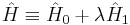
Starting with the one-particle Dirac equation written earlier with and rewritten here as:

where  is the
  unit matrix. This Hamiltonian is rewritten, namely divided into two parts:
where
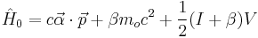
and
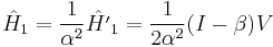
where  is the Fine-structure constant (not to be confused with the Dirac alpha matrices). Letting
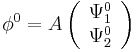
into the zero order equation for and using a particular but known representation of the Dirac operators, yields:
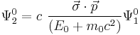
where  are the
  Pauli matrices. Note that the potential
  does not appear in the equation above. The equation for the other spinor is:
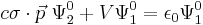
where 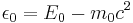 . Eliminating
  gives:
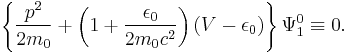
This is simply the non-relativistic equation for a system with a re-normalized potential and energy eigenvalue:
The higher-order corrections can be obtained by conventional perturbation theory. This is known as Moore's decoupling technique. Though it resembles the FW transformation, it is computationally and conceptually much simpler. Though misunderstood at first, in part because the fine structure constant appears in both the equations and the order parameter  requiring care in the "bookkeeping" of the perturbative scheme, Moore's decoupling technique was vindicated for the (relativistic) hydrogen atom using conventional Rayleigh Schrödinger perturbation theory and computer algebra and proven to converge to the correct solution [1]. It has been applied successfully to relativistic calculations on Alkali metals and represents one of many relativistic perturbative schemes investigated by Werner Kutzelnigg[2][3].
Notes
- ^ T.C. Scott, R.A. Moore, G.J. Fee, M.B. Monagan and E.R. Vrscay, "Perturbative Solutions of Quantum Mechanical Problems by Symbolic Computation", J. Comp. Phys., 87, 366-395 (1990). [1]
- ^ W. Kutzelnigg,"Perturbation theory of relativistic corrections. II. Analysis and classification of known and other possible methods.", Z. Phys. D 15, 27 (1990).
- ^ W. Kutzelnigg,"Perturbation theory of relativistic effects", in Relativistic Electronic Structure Theory, Part I, P.Schwerdtfeger ed. Elsevier (2002).